Bayes’ Theorem is one of the most widely used and celebrated concepts in statistics. It sets the basis of a probability theory that allows us to revise predictions or hypotheses based on new evidence.
In a previous article on probability notations (1, 2), I introduced P(B∣A)— the probability of event B happening given that event A has already occurred.
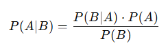
Bayes’ Theorem flips this perspective, focusing on P(A∣B): the likelihood of A, given that B has occurred. In essence, it helps us refine our understanding of outcomes by incorporating prior information (known data).
In practice, even if your initial assumptions or estimates aren’t perfect, the process of applying the Bayes’ theorem encourages more thoughtful and informed guesses for the future!
To begin with, let’s look at an example inspired by the famous work of Daniel Kahneman and Amos Tversky.
Table of Contents
- Example
- Applying Bayes’ Theorem Intuitively
- Applying Bayes’ Theorem Mathematically
- A different look at Bayes’ Theorem
- Real-Life Applications
- Summary
1. Diana: A Hypothetical Scenario
My friend recently matched with a girl named Diana on a dating app. After chatting for a while, he describes her as someone with a keen eye for detail, an open-minded personality, and a direct yet understanding communication style. She seems friendly, but a bit shy and quiet.
Based on this description, let’s pose a question:
Is Diana more likely to be a library assistant or a soccer player?
At first glance, you might be tempted to say “library assistant” based on the stereotypical traits associated with the description. And you’re not alone! In a similar experiment conducted by Kahneman and Tversky, 85–90% of participants chose the “library assistant” option.
But there’s a catch (Theres always a catch).
The Statistical Trap
Kahneman and Tversky’s research highlights a critical oversight: most people ignore base rates — the actual ratio of library assistants to soccer players. Statistically speaking, there are far more soccer players than library assistants in the population. This omission often leads to flawed judgments.
Of course you may say this test is flawed because no prior information is given or you didn’t tell us the specifics, etc.
But, in real-world applications as a data scientist… this teaches us an important lesson: Before answering questions or making predictions, we must carefully consider the relevant factors and incorporate prior probabilities.
2. Applying Bayes’ Theorem Intuitively
Let’s revisit Diana’s example, but this time, we’ll apply Bayes’ Theorem.
We sought out to gather 1,000 individuals randomly from a group that only had library assistants or soccer players. We got from this group
- 50 library assistants (5%)
- 950 are soccer players (95%)

Based on our description of Diana, we estimated that 40% of library assistants and 10% of soccer players match Diana’s description.
- Library Assistants Matching the Description: 50 × 0.40 = 20
- Soccer Players Matching the Description: 950 × 0.10 = 95
From this data alone, we can technically calculate the probability of a person being a library assistant (L) given the description (D), noted as P(L | D).
Use your Intuition
Okay, I haven’t given any equations regarding the Bayes’ Theorem yet. However, we’ve almost been able to answer this question intuitively instead of looking at mathematical formulas.
In order to find the probability of a person being a library assistant given the description… We would divide the number of library assistants matching the description (20 library assistants) with the total number of people (both soccer players and library assistants) that match the description (115 people).

- 20 library assistants match the description
- 95 + 20 = 115 total people match the description
The Insight
Contrary to intuition, the 17.4% shows that Diana is statistically more likely to be a soccer player despite her description aligning more closely with a library assistant stereotype! Even if you think that Diana’s description likely fits to be a library assistant 4 times more than a soccer player (40% vs 10%), it’s not enough to overcome the fact that there is just a much greater number of soccer players in the population
This is why we must carefully consider the relevant factors and incorporate prior probabilities.
3. Bayes’ Theorem (Mathematically)
Okay, since we got the intuitive part out of the way, let me give you the mathematical explanations of the Bayes’ Theorem. In the introduction, I mentioned that Bayes’ Theorem flips the perspective to focus on P(A∣B)— the probability of A occurring given that B has happened.
But if you’re like me, you might find the standard “event A” and “event B” notation a bit abstract and confusing at first.
If you’ve ever wondered:
- What exactly qualifies as “event A”?
- How do we define “event B” in practical terms?
Congratulations — you’re likely among the 95% of people who probably had the same questions when studying probability. So, for me, after studying and looking around for different ways to understand… I found a solution to wrapping my head around these notations.
Hypothesis (H) and Evidence (E): A Better Way to Understand
I’ll introduce you guys to looking at Bayes’ Theorem in terms of Hypothesis (H) and Evidence (E) instead of the generic event A and event B. This framing makes it easier to apply the theorem in real-world scenarios.
If we just go back to our example:
- Hypothesis (H): What you are trying to assess or predict (Chances that Diana is a library assistant.)
- Evidence (E): The observed data or information that could support or refute the hypothesis (40% of library assistants and 10% of soccer players match Diana’s traits)
What we want to solve is the probability of the hypothesis being true given that the evidence is true. We can actually mathematically label this as:
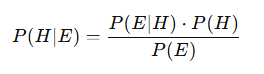
- P(E ∣ H): The probability of observing the evidence E if the hypothesis H is true (likelihood).
- P(H): The prior probability of the hypothesis H before observing the evidence.
- P(E): The overall probability of the evidence E under all possible hypotheses.
If we think about it in terms of the hypothesis we are making and the evidence (data) that we have, it becomes much more straight forward in answering these questions!
If you made it this far into my article, I would appreciate it if you could leave a few claps :). It helps me get motivated to write more educational content!
4. Bayes’ Theorem with Example
Let’s walk through how we calculated probabilities in our earlier intuitive approach, but this time using the formal framework of Bayes’ Theorem.
Recall that we have 1,000 people in our dataset: 50 library assistants and 950 soccer players. Out of these, we estimated that 40% of library assistants and 10% of soccer players match Diana’s description.
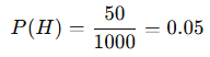
How can we find our P(H)?
The prior probability, P(H), is the probability of the hypothesis (Diana being a library assistant) before considering any evidence. This means asking:
If we know nothing about Diana, what’s the chance she’s a library assistant in this group?
Well.. that would simply be..

How can we find our P(E | H) ?
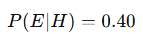
P(E∣H) is the probability of observing the evidence (Diana’s description) assuming the hypothesis is true (Diana is a library assistant).
If we limit our view to only library assistants, 40% of them fit Diana’s description. Thus:

How can we find our P(E)?
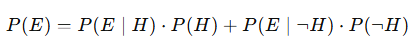
The marginal probability of evidence, P(E), is the total probability of observing the evidence E, considering all possible hypotheses.
This is where we account for both library assistants and soccer players matching the description.
Using the law of total probability:


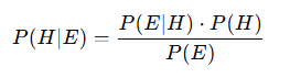
Final Calculation Using Bayes’ Theorem
Now, we can calculate P(H∣E), the probability that Diana is a library assistant given the evidence:
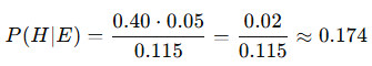
Hey, look at that! The probability that we obtained is the same as the probability that we obtained from our intuitive approach!
Understanding Bayes’ Theorem in Practice
It’s been all just equations and theoretical understandings so far in this article. However, Bayes’ Theorem has a lot of practical applications in updating our beliefs based on new evidence. So, let me ask you a question:
Why or How do we use Bayes’ Theorem in practice?
Think about this: What does P(H∣E) or “the probability of our hypothesis being true given the evidence,” really mean? I’d say that the Bayes’ Theorem helps us refine our hypothesis — or our belief about something — based on the strength of the evidence at hand.
With that in mind, let’s think about a practical example from the perspective of a data scientist at a biotech company.
Evaluating the Effectiveness of a New AIDS Drug
Imagine you’re working at a biotech company developing a new AIDS drug. Your goal is to determine if this drug is effective based on the data collected from clinical trials. In this scenario, you want to calculate P(H ∣ E) — the probability that the drug is effective (our hypothesis, H) given the data (our evidence, E) from the trials.
1. Prior Probability, P(H)
This would be your belief about the probability that the drug is effective before analyzing any data. It is often informed by historical data, expert opinions, or subjective judgment (be careful with subjective judgments).
- Based on historical trends, only 20% of new AIDS drugs turn out to be effective: P(H)=0.2
2. Likelihood, P(E∣H)
This is the probability of observing the data (E) if the drug is truly effective (H). It’s derived from trial results, such as patient outcomes.
- Here, the drug improves outcomes in 90% of cases when effective: P(E∣H)=0.9
3. Probability of Data Given Ineffectiveness, P(E∣¬H)
This is the probability of observing the data even if the drug is not effective (¬H). It’s often informed by control group data, such as the placebo effect.
- Here, the drug improves outcomes in 30% of cases when not-effective (from random chance or placebo): P(E∣¬H)=0.3
Marginal Probability, P(E)
This accounts for the probability of observing the data (E) regardless of whether the drug is effective or not. It’s calculated using the law of total probability:
From our calculations, P(E) = 0.42.
Calculating P(H∣E)
Now that we have all the components, we can calculate the probability that the drug is effective given the observed data:

Bayes’ Theorem in this case updated our beliefs in light of new evidence. There’s about a 42.9% chance the drug is effective based on the data.
- Before observing the data: We had a 20% belief in the drug’s effectiveness.
- After analyzing the data: That belief increased to ~42.9%.
However, the evidence isn’t overwhelming, emphasizing the importance of collecting additional data to make well-informed decisions.
Note: You can imagine why 42% isn’t satisfactory right?
Summary
I’ll go back to the phrase that I began this article with.
In practice, even if your initial assumptions or estimates aren’t perfect, the process of applying the Bayes’ theorem encourages more thoughtful and informed guesses for the future!
What makes Bayes’ Theorem so powerful isn’t just its ability to deliver accurate probabilities — it’s about how it offers a structured way to think critically about uncertainty.
Whether you’re a data scientist evaluating drug efficacy, a business leader making strategic decisions, or simply someone interpreting real-world scenarios, Bayes’ Theorem helps you integrate new information without losing sight of the bigger picture.
I hope the examples with Diana and the Biotech company helped clarify how Bayes’ Theorem works in real-world contexts and why it’s such a valuable tool. It’s not just about avoiding statistical traps — like ignoring base rates — but also about making smarter, more informed decisions.
I hope you were able to learn something!
P.S: If you are looking for a continuation of the Bayes’ Theorem and how it is used in classification for machine learning, I recommend my article on the Naive Bayes!